
Indoor Localization with Wireless Networks
During the summer of 2018, I had the opportunity to work for the telecommunications corporation NEC in Sendai, Japan on a project that focused on indoor localization using wireless networks. This partnership was made possible by IPAM’s GRIPS program which pairs graduate students in mathematics with corporations in places like Berlin, Germany and Sendai, Japan to solve problems in biotechnology, transportation, and telecommunications. Unlike the usual signal processing paradigm I work in where the aim is to recover a signal given certain measurements, localization focuses on recovering the location of where a signal is transmitted given certain data. Most people are familiar with Global Positioning System (GPS) which makes navigating roadways with Google Maps possible. Most people are also undoubtedly aware of the shortcomings of GPS in sheltered environments like parking decks or office buildings. The reason this is the case is that GPS relies on your smartphone having line of sight, or an unobstructed view, of at least four satellites used for GPS. When this is not the case, localization error can be several meters large.
Certainly for most navigation purposes GPS suffices, but it’s also easy to imagine instances when we need navigation in environments where our smartphone does not have line of sight with any GPS satellites. For example, you might wish to find your favorite store in a large indoor shopping complex. The applications of indoor localization go far beyond this simple example though. Advertisers in particular are interested in accurate localization estimates for creating localized advertisements. Emergency response teams are also interested in localization, as they could find victims trapped inside a partially destroyed or obstructed building. Perhaps the most impactful application of indoor localization is with the internet of things (IoT). NEC is most interested in this setting, as they work with security firms and production facilities who are interested in automating certain tasks.
There is a rich literature on indoor localization. Liu and Davidson give a nice summary of what has been done so far. A non-exhaustive list of the most prominent data that one can use for localizing includes time of flight (ToF), angle of arrival (AoA), and received signal strength (RSS). ToF is, as you might expect, the time it takes for the signal to travel from the transmitting device to the receiver. AoA is the angle that the transmission makes relative to the receiving antenna(s). Received signal strength is, as the name suggests, a measure of signal strength that the receiver obtains from a particular transmission, typically from a wireless access point or router. There are other technologies that one can use such as channel state information or Bluetooth. However, current wireless network infrastructure limits our options down to RSS. RSS is ubiquitous because any device adhering to the IEEE 802.11 protocol has RSS data embedded in the packets, or the basic unit of wireless communication, it sends.
The problem with RSS is that it is an incredibly sensitive variable. First and foremost, it’s not a standardized measurement in terms of units. Different devices can have different units for RSS. Further complicating matters is that signals transmitted in indoor environments are prone to a variety of environmental factors which can distort RSS at a surprising scale. Multipath propagation, or the phenomenon where a signal “bounces” off the walls, can cause a signal to interfere with itself in non-obvious ways. Not only does it depend on the geometry of the indoor environment, but the composition of materials also matters. Different materials can cause a signal to attenuate at different rates. This is particularly important when a signal transmission does not have line of sight with a receiving antenna. How the transmitting antenna is oriented, or how you hold your smartphone, with respect to the receiving antenna also has a non-trivial impact on RSS values.
To the best of my knowledge, there are two methods using RSS which allow one to estimate the location of a signal transmission. The first is a method known as fingerprinting. Fingerprinting is a method which consists of an offline phase and an online phase. During the offline phase, RSS measurements are recorded at predetermined locations called reference points in a particular indoor setting. These measurements along with their distance to each wireless access point are then stored in a database which is sometimes referred to as a “radio map”. During the online phase, RSS values are compared to those stored in the database and the position of a transmission is estimated based on which database entry is most similar to the online measurement. These measurements are understandably very tedious and expensive to collect. Further, the database of RSS measurements degrades in quality as the indoor environment changes. Nevertheless, fingerprinting appears to be the state of the art in terms of localization methods which rely solely on RSS.
The other paradigm of localizing with RSS includes approaches which use path loss models. Path loss models are motivated by the physics of signal attenuation in simple environments. To give a specific example, the Friis free space equation says that the power of a transmission with no multipath propagation and with line of sight decays according to the law \[ \begin{align} P_{loss} = \left(\frac{c}{4\pi f d}\right)^2, \end{align}\] where \(c\) is the speed of light, \(f\) is the frequency of the transmission, and \(d\) is the distance the transmission travels. More general path loss models might incorporate random variables to model signal fading or might adjust the exponent in the above expression to account for cases when there is no line of sight or when there is multipath propagation. For reasonable devices, such as the Raspberry Pi 3, where RSS is a function of the signal power it’s easy to use this formula to estimate the distance a transmission from a wireless access point travels. The simplicity of path loss models is both a blessing and a curse. First and foremost, they require very little calibration to specific indoor environments. Distance estimation is also very easy to compute with just a little bit of algebra. However, path loss models often understate the complexity of indoor environments and consequentially suffer localization errors of several meters.
A Dynamic Path Loss Model
The laundry list of factors which influence RSS measurements along with the difficulty of getting sub-meter localization error with the above methods has led many researchers to conclude that the future of indoor localization will likely rely on additional forms of data to estimate a transmission’s position. Nevertheless, NEC tasked my colleagues and me with producing a new approach to indoor localization using RSS measurements in just 2 short months. Our group recognized that fingerprinting was ultimately an unsustainable solution so we decided to focus on improving the shortcomings of path loss models. In our case, NEC provided us with Raspberry Pi 3’s and a particular router which gave us RSS measurements in dBm. This was nice since signal power and RSS in this case are related by the simple transformation \(RSS = 10\log_{10}(P)\). Skipping some details which you can find in the surveys linked to above, this meant that our basic path loss model at time \(t\) is of the form \[ \begin{align} RSS(t) = T_x - 10n\log_{10}(d(t)), \end{align}\] where \(T_x\) is the transmission power in dBm from 1 meter’s distance and \(n\) is the path loss exponent which is to be chosen based on the indoor environment. Engineers seem to have some rule of thumb which governs how to choose \(n\) in various contexts. However, existing models choose \(n\) once and it is fixed thereafter.
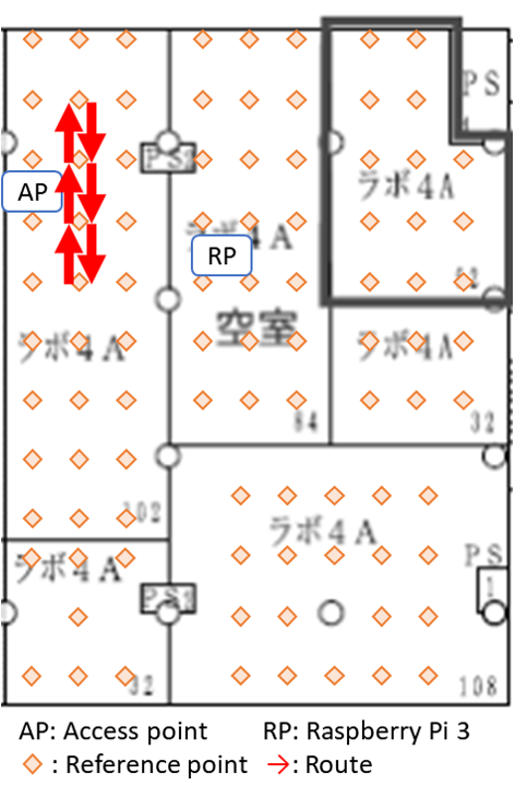
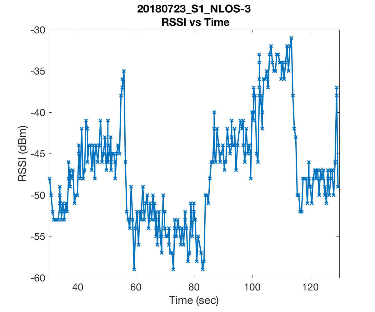
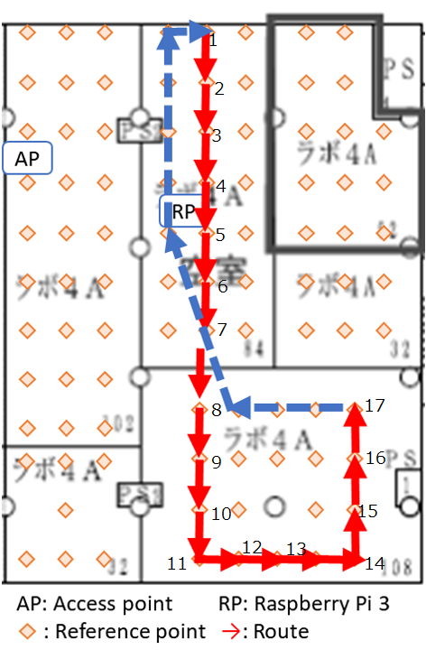
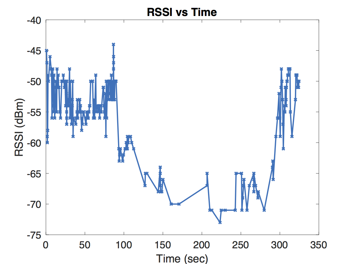
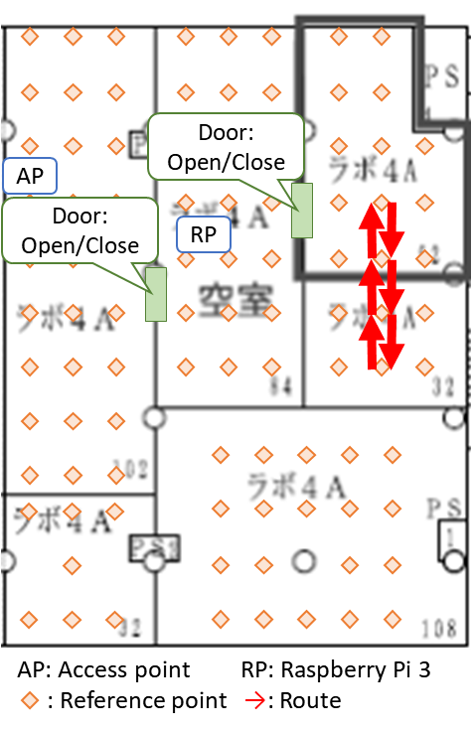
Since indoor environments often consist of many rooms with different layouts, we conjectured that a path loss model which dynamically adjusts its path loss exponent may better capture the complexity of certain indoor settings. The question of when and how to adjust the path loss exponent was based on some experiments that we conducted in our office. Our office consisted of six rooms which we partitioned into three sections named S1, S2, and S3 listed in decreasing order based on their average distance to the lone access point, or router, we had (pardon the pun) access to. We laid a uniform grid of reference points spaced 2 meters apart from each other and collected measurements on a subset of these reference points. Below are a few figures which illustrate some of the paths that we walked, indicated in red arrows, and the recorded RSS measurements at various times. In the figures, AP is the location of the access point and RP is the location of the Raspberry Pi that we used to monitor, or “sniff”, packets. The other Raspberry Pi was held in our hands as we walked along the paths.
| Route | RSS Measurements | |
|---|---|---|
 |
 |
|
 |
 |
|
 |
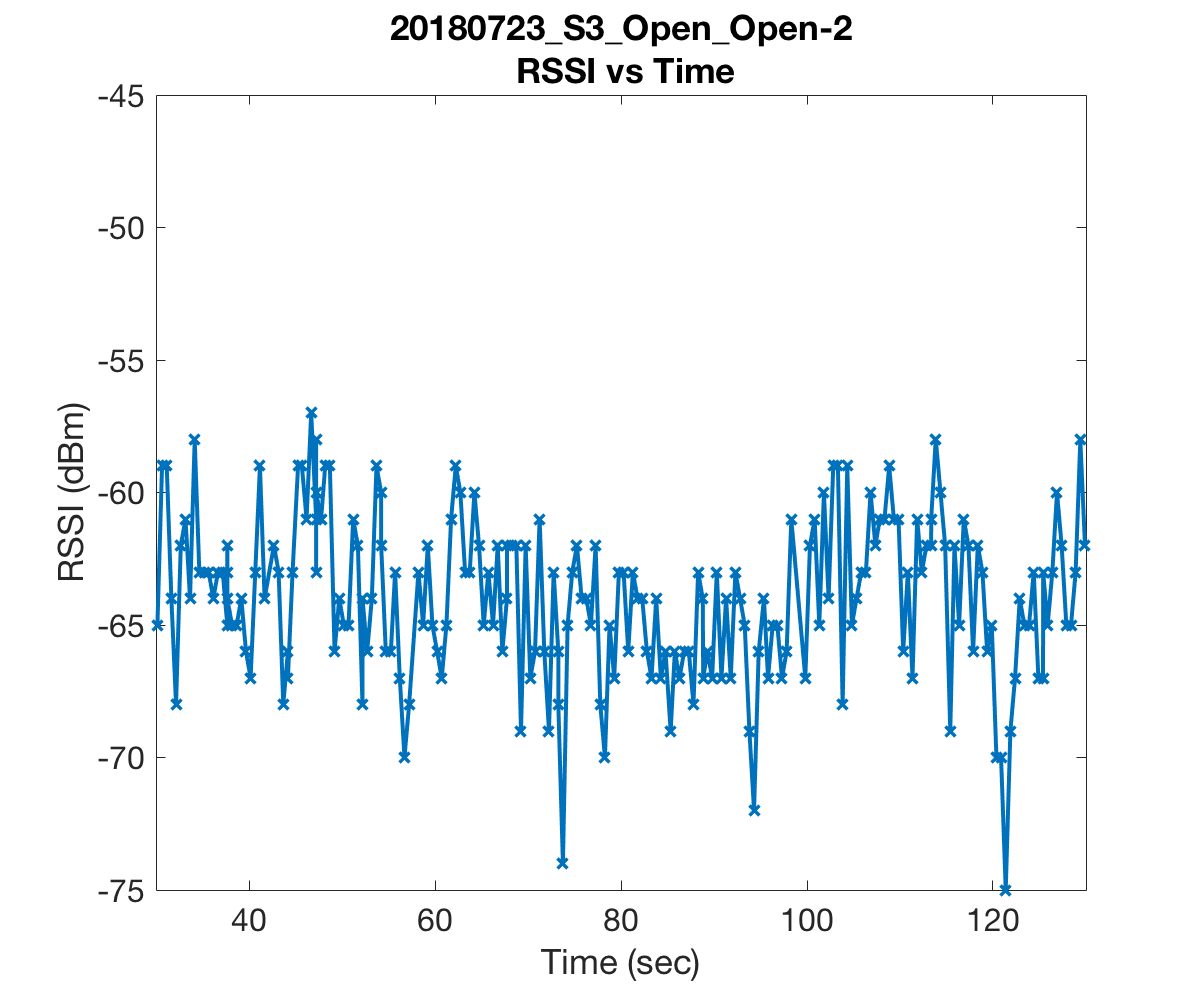 |
The first two figures substantiate the claim that RSS is indeed a rather volatile beast. We were alarmed to see that readings could drop as low as -60dBm just a few meters from the access point. These measurements were as low if not lower than those we recorded in the room most far removed from the access point. Further, the drops in RSS in the first plot were due simply to obstructing the line of sight by a computer monitor and one of our colleague’s bodies!
The model our group ultimately decided upon adjusts the path loss exponent at times when the RSS curve experienced sharp jumps. This dynamic model can be broken down into two pieces, namely jump detection and distance estimation.
Jump Detection
The hardest part of jump detection is defining what a jump is. I’m not sure we ever decided on a formal definition. A formal definition would likely be overly restrictive or too vague to be useful anyways. Me being me though, wavelet coefficients were the first candidates for detecting discontinuities in RSS of various sizes and over various time intervals. The above plots demonstrate that RSS naturally fluctuates about some piecewise-smooth curve governed by the path a user takes while holding their Raspberry Pi. To ignore these small and spurious jumps we needed some way of denoising our signal. Our first guess was to apply some low-pass filters to our data, but the problem with applying low-pass filters is that we have to choose a stop band, or which frequencies to treshold out. Unfortunately, when we compared the power spectra of various RSS curves it appeared to be the case that the severity of the signal’s non-line of sight strongly influences the spectrum of our signal. This suggested that we might have to choose a dynamic stop band which would further add to our quickly growing list of parameters to choose.
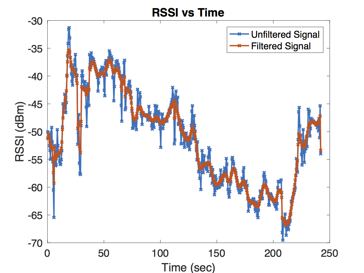
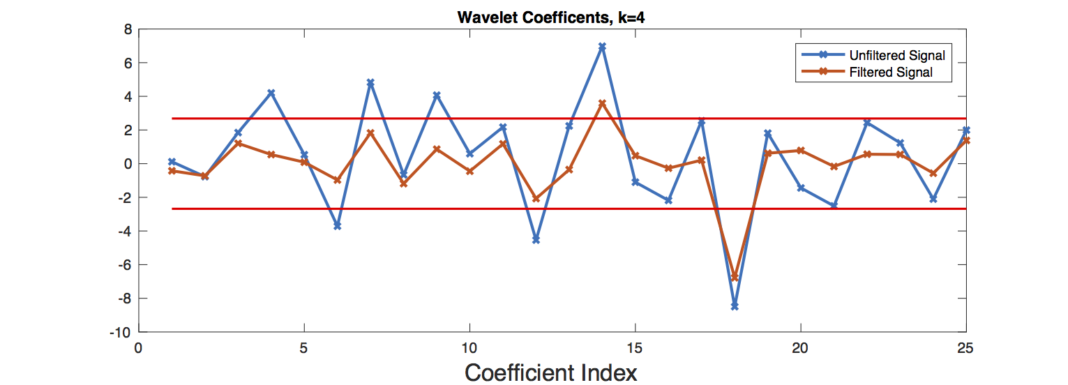
The simplest and most effective model for denoising ended up being Donoho’s and Johnstone’s RiskShrink which shrinks empirical wavelet coefficients under the assumption that the signal is perturbed by Gaussian noise. A comparison of filtered and unfiltered RSS curves is shown below. For this example, wavelet coefficients at scale \(k=4\) were filtered. Since this experiment was sampled at a rate of \(2\)Hz, \(k=4\) corresponds to a time scale of 8 seconds.
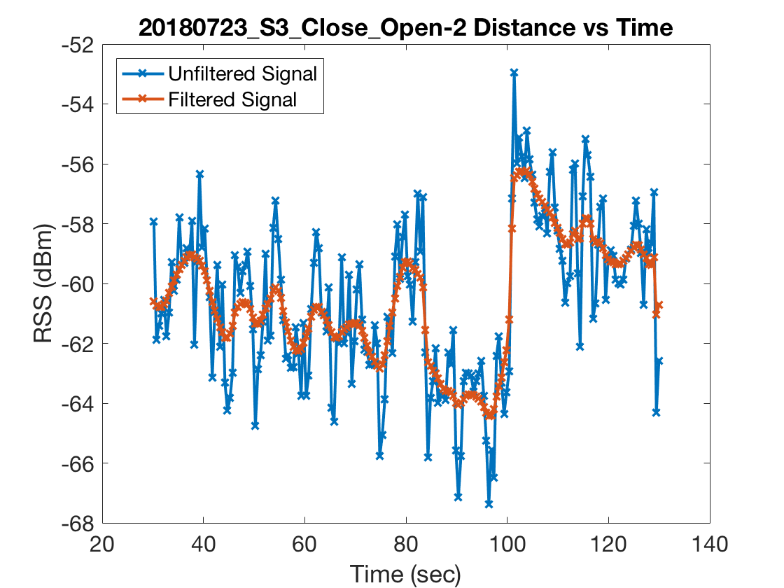
Next we needed a procedure for selecting significant wavelet coefficients from the filtered RSS curve which we would label as jumps. We used the difference between the unfiltered and filtered RSS curves as a model for noise and chose the \(1-\alpha\) percentile of the noise’s wavelet coefficients as the threshold for significant wavelet coefficients. Choosing \(\alpha\) by cross validation is probably the best option but we had so few experiments–39 to be exact–that we stuck with a value of \(\alpha = 20\). In practice this seemed to work quite well on the handful of experiments we conducted where we carefully monitored the transitions between line of sight and non-line of sight settings. Below are two figures which plot RSS measurements from a particular experiment along with the wavelet coefficients of the filtered and unfiltered RSS curves as well as the threshold plotted in red.
Comparing Dynamic Model to Static Model
We could have spent more time on perfecting jump detection, but with what little time we had remaining we decided to move onto estimating distance from our access point using our dynamic model. Recall that our model assumes \[ \begin{align} RSS(t) = T_x - 10n\log_{10}(d(t)), \end{align}\] where \(n = n(t)\) is really a function of previous RSS measurements. We essentially adjust \(n\) linearly with respect to the net change in RSS during a jump. That is, for some predetermined \(\beta\) and an interval \([t_0, t_1]\) over which a jump occurs we set \[ \begin{align} n(t_1) = n(t_0) - \beta(RSS(t_1) - RSS(t_0))\end{align}.\] Other than \(\beta\), one has to choose an initial pass loss exponent.
To compare how much of an improvement the dynamic model offers over static path loss models, or those with a fixed path loss exponent, we initialized both dynamic and static path loss models with a path loss exponent that was chosen by cross-validation under \(\ell_2\) loss. More formally, letting \(f_i, g_i\) denote the vectors of predicted and true distances respectively with length \(m_i\), we define the risk to be \[ \begin{align} \sigma &= N^{-1} \sum_{i=1}^{N} L(f_i, g_i),\newline L(f_i, g_i) &= \left(m_{i}^{-1} \sum_{j=1}^{m_i} (f_i(j) - g_i(j))^2\right)^{1/2} \end{align}.\]
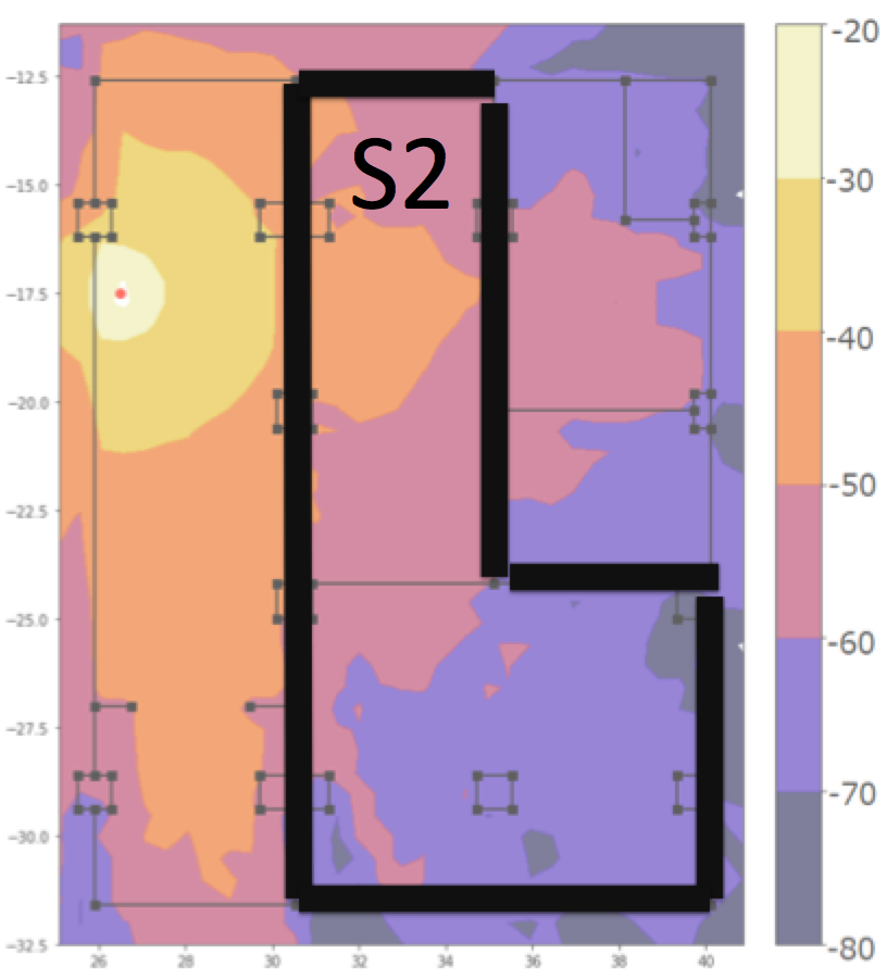
We were initially surprised when we trained our dynamic path loss model that it offered a meager improvement in risk over the static model by \(7\) millimeters. Upon further reflection we realized that this is likely due to the fact that our experiments are a bias data set. Only 6 of our 39 experiments had a path that transitioned between regions of good and poor signal coverage. All 6 of those regions happened in S2 of our office. See the below figure for a heat map–generated by an algorithm developed by my colleagues Shizuki Goto, Ryoichiro Hayasaka, and Hannah Horneh– of wireless signal strength as well as a precise definition of what S2 of our office is.
When we retrained our dynamic model on each section of our office, we found that the dynamic model offered the following improvements in risk over the static model.
| Region | Static Risk | Dynamic Risk |
|---|---|---|
| S1 | 1.44m | 1.40m |
| S2 | 3.71m | 2.19m |
| S3 | 1.13m | 0.95m |
The actual performance is of course a bit more nuanced than what these estimates for the risk suggest. While the dynamic model on average performs better than the static model in terms of risk, it’s worth illustrating some extreme examples to show what works and what needs improving. Take a look at the following experiments along with the predicted and true distances.
| Route | Distance Estimation | |
|---|---|---|
|
 |
|
|
 |
|
|
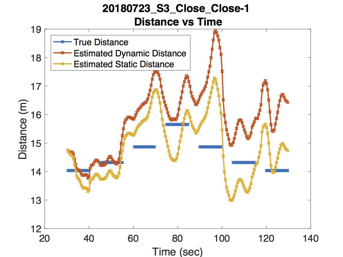 |
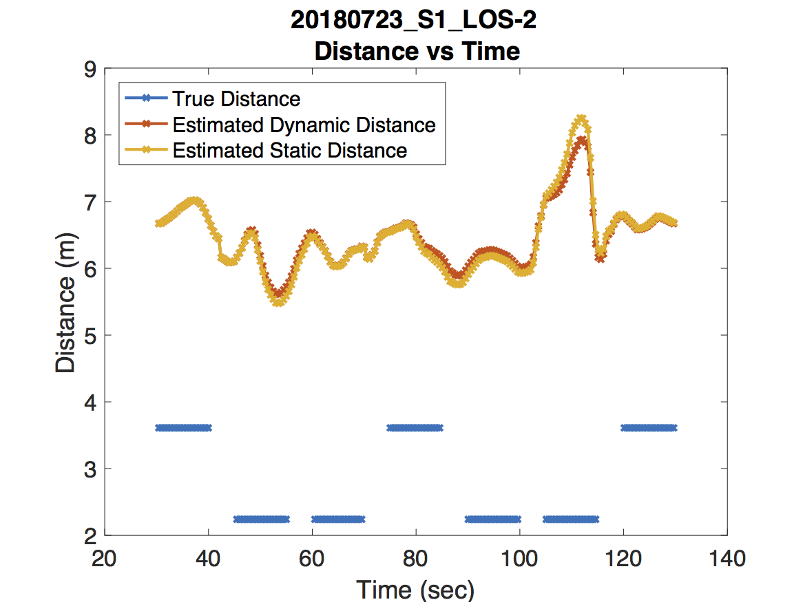
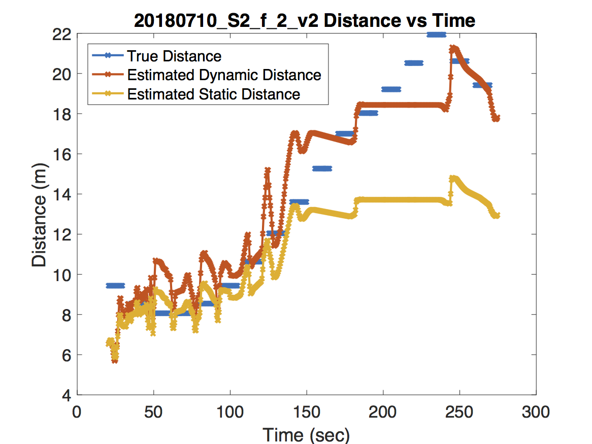
For the experiment in the first figure, the Raspberry Pi was held above one of our colleague’s heads to maintain line of sight with the access point. As expected, the dynamic model deviates very little from the static model. For the experiment in the second figure, our jump detection algorithm correctly detects a sharp jump due to a room change. Because the wireless coverage in each room are dramatically different, adjusting the path loss exponent leads to a much more accurate distance prediction. Finally, the experiment in the third figure never obtains line of sight. There are some small jumps that occur due to orienting the Raspberry Pi in the direction of the access point and changing rooms. However, our jump detection algorithm misses a jump around 55 seconds which causes an error in the dynamic model’s distance estimation. Unfortunately this error propagates forward in time.
Concluding Remarks
It appears then, perhaps unsurprisingly, that our dynamic path loss model is only as good as the jump detection algorithm. I think there are improvements that could be made to make the advantages of the dynamic path loss model more pronounced. In particular, I think having more access points and therefore more RSS curves could allow coordinated jump detection. Since the dynamic path loss model improves upon the static model when a transmitter crosses the boundary of “good coverage” for an access point, having more boundaries seems like an obvious way to increase the performance of the dynamic model. Besides, for most commercial indoor settings there will be several access points scattered throughout.
Another improvement that could be made is detecting jump across finer time scales. For simplicity our jump detection algorithm only looked at classifying wavelet coefficients at one scale, roughly corresponding to 5 seconds. Looking at a variety of time scales might prevent the jump detection algorithm from missing jumps. The caveat to this of course is that the signal to noise ratio at smaller scales will be much smaller than at higher scales.
For anyone who is interested in the details of this project as well as the code used for jump detection and distance estimation you may find a project write up as well as MATLAB code on my GitHub account here.
After working on this project for two months, I’m inclined to agree with the existing literature that the future of indoor localization will require methods that rely on additional forms of data other than RSS. There appear to be fundamental limitations to how much information can be extracted from RSS. While I think methods like dynamic path loss models can mitigate the error due to erratic discontinuities in RSS measurements, fingerprinting and path-loss models are far from sub-meter accuracy which is required in certain settings like automation in factory settings.