An Overview of Blind Deconvolution

Motivation

I remember as a first year student at UGA I was enrolled in a multivariable mathematics class. At the time that class was impossibly difficult for me, but looking back I’m grateful for enrolling in it. A lot of key ideas that I would see later in my academic career had seeds that were planted during that first year. As a matter of posterity, the lectures of this course were recorded and made publicly available on YouTube courtesy of Patty Wagner, yours truly, and a few of my then colleagues. The professor of that course, Ted Shifrin, who is a good friend and mentor of mine now, is famously known by his students for incorporating geometry to a mathematical discussion whenever he finds the chance to do so. An extreme example of this is demonstrated by an Abstract Algebra text he authored titled “Abstract Algebra: A Geometric Approach.”

I particularly remember working on some homework problems involving conic sections and coming across a problem which outlined the mathematics behind what are known as “whispering galleries.” Effectively these are rooms in the shape of an ellipse where two speakers can whisper to one another from across the room and hear each other perfectly clear. This is possible due to the nature of how sound waves propagate and reflect off surfaces. If you click on the link, you’ll see a neat gif illustrating this phenomenon.

It’s worth re-emphasizing that whispering galleries only work due to the very special geometry of the room. Anyone who has tried having a conversation with a friend or colleague from across any normal room knows that a whisper likely isn’t going to be heard. On the other extreme one can imagine being inside a large vacant room and shouting towards the other person. The problem with this latter scenario is that, depending on the material that the room is composed of, you’re likely going to hear a lot of echoes which makes discerning what was said difficult.

If you’ll humor me, imagine someone gives you a recording of someone talking in some unknown room where there are lots of echoes and reverberations and asks you what the person was saying. You might be able to piece together bits of what was said but if the recording is so poor due to the echoes you can imagine that the recording might be entirely uninterpretable. This problem of getting rid of echoes is formally known as blind deconvolution.

The above example may seem artificial but, in fact, the scope of problems which can be classified as blind deconvolution is expansive. One important example is medical and astronomical imaging where the goal is to deblur a noisy image. Another example is communications engineering such as for the Internet of Things and for 5G networks where multiple devices are communicating with a single base station.

A Mathematical Model

Let’s return to the example of a person speaking to a single microphone in a room with poor acoustic design. As the person speaks the sound waves from the speech emanate across the room, echoing off walls, and after some time reach the microphone. Let’s call the function encoding the amplitude of the sound wave of speech \(x(\cdot)\), where the argument of the function is time.

Now, if the microphone and the person were in a room with no wall then the microphone at time \(t\) would simply hear \(x(t)\) or perhaps a delayed signal \(x(t-\tau)\) accounting for the time it takes for the sound wave to reach the microphone. When we add walls the picture is much more complicated.

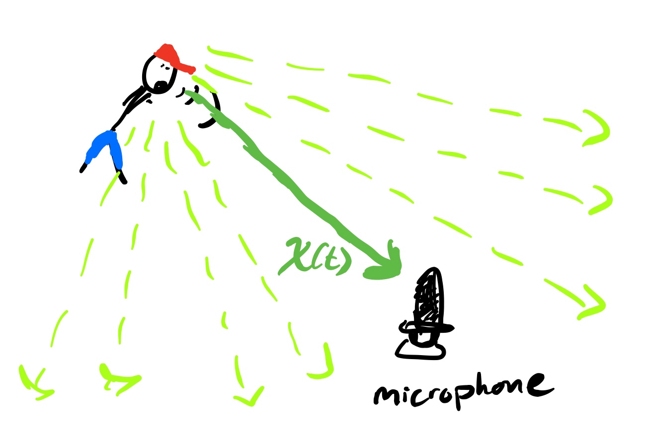Fig. 1: A cartoon illustrating how sound propagates in free space.

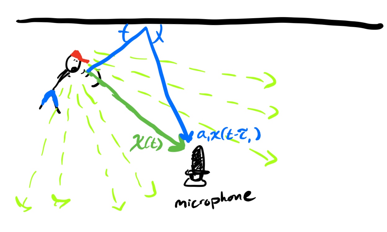Fig. 2: A cartoon illustrating how sound propagates in a space with one wall. Notice there will be a single echo off this wall reflecting back to the microphone.

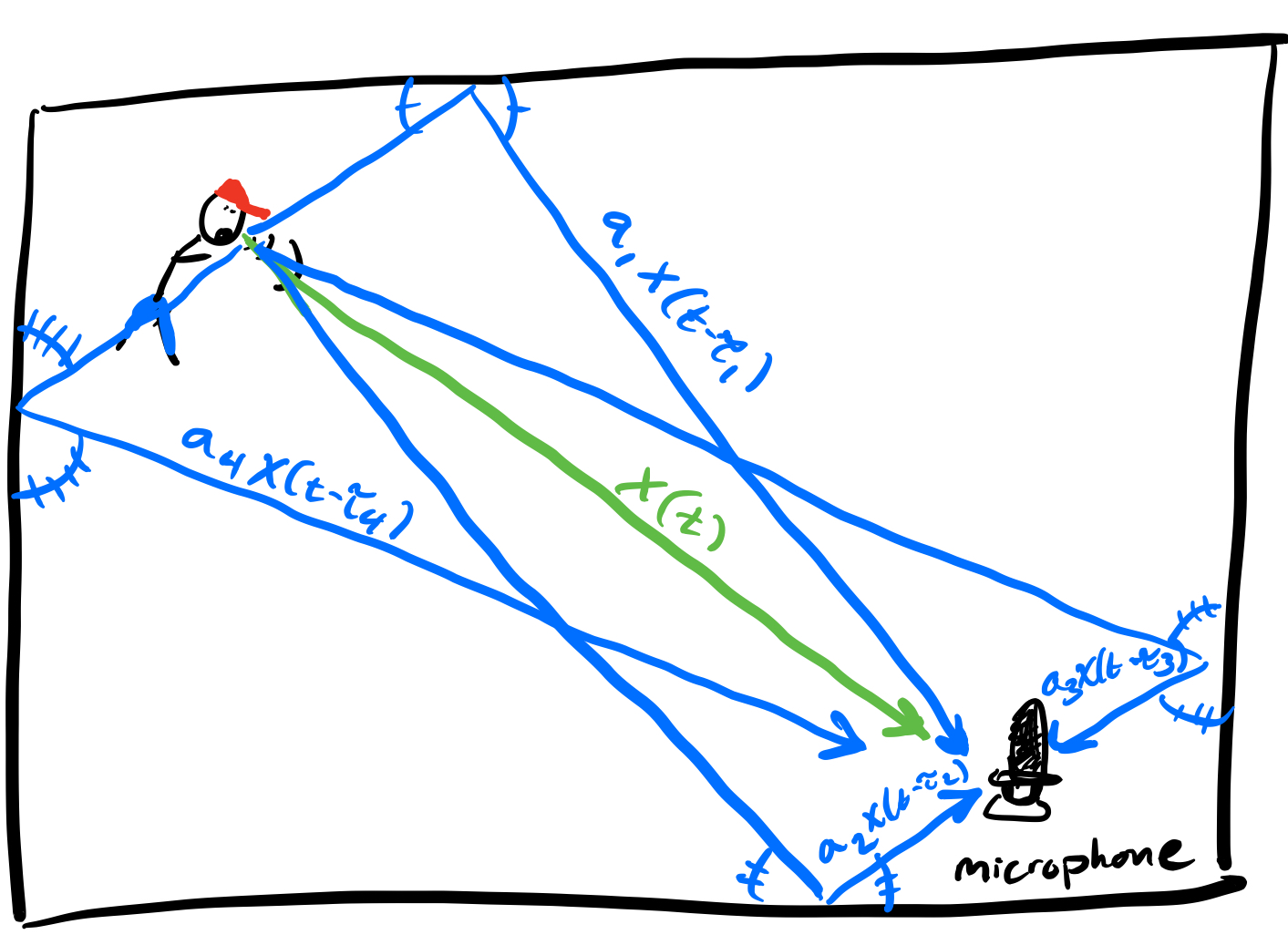Fig. 3: A cartoon illustrating how sound propagates in an enclosed room with a rectangular layout. Only the direct propagation and “single echo” propagations are sketched, but in general sound can echo off many walls before reaching the microphone. This is the infamous multipath propagation phenomenon that made the indoor localization project so challenging.

When sound waves echo off a surface they will attenuate or dampen as a function of the material they echo off of. Let’s model that by multiplication by some scalar. That is, after reflecting off of some fixed wall the echoed sound wave is now \(a \cdot x(\cdot)\). So if the person and the microphone were in an open space with one wall nearby then at time \(t\) the microphone would hear the sound travelling directly from the speaker \(x(t)\) but also the sound coming from the echo off the wall of an earlier part of speech \(a \cdot x(t-\tau)\), where the shift comes from the time it takes the sound wave to travel the extra distance from the speaker to the wall and the wall to the microphone. In other words, if we denote the amplitude of the soundwave received by the microphone at time \(t\) as \(y(t)\), we have \(y(t) = x(t) + ax(t-\tau)\).

Now when there are multiple walls there are many ways for the sound wave \(x(\cdot)\) to echo off and reflect back to the microphone. Technically speaking the sound wave could echo off an arbitrarily large number of walls before reaching the microphone. In effect that means at time \(t\) the microphone would receive

\[ \begin{align} y(t) = \sum_{i=1}^{n(t)} a_i x(t - \tau_i). \end{align}\]

I’m a digital signal processor, so let’s assume that we’ve discretized time and that our original signal \(x(\cdot)\) is now represented by a vector in \(\mathbb{R}^L\). If we store our attenuation coefficients, or our filter, in a vector \(a \in \mathbb{R}^L\) then we can rewrite the equation above as

\[ \begin{align} y_j = \sum_{i=1}^{L} a_i x_{i\ominus j} = (a * x)_j, \end{align}\]

where \(\ominus\) denotes circulant subtraction modulo \(L\) and \(*\) denotes circulant convolution.

So this explains part of the reason why this problem is called blind deconvolution. The reason for the world “blind” is because a priori we know neither \(a\) or \(x\)! We don’t know \(a\) because we don’t have information regarding the composition of the room, and we don’t know \(x\) because that’s the speech we’re trying to retrieve from the recording \(y\).

A Compressed Sensing Approach

Whenever mathematicians see convolutions immediately their spidey senses tingle telling them that the natural thing to do is take a Fourier transform. Indeed, any first year math graduate student who has taken real analysis can tell you that the Fourier transform turns convolution into point-wise multiplication, namely

\[ \begin{align} \hat{y}_j := (Fy)_j = (Fa)_j (Fx)_j =: (\hat{a} \odot \hat{x})_j. \end{align}\]

Even with this nice reformulation of the problem it’s still viciously ill-posed for a couple of reasons. First, if \(\alpha\) is any non-zero complex number, then \(\hat{y} = (\alpha \hat{a}) \odot (\alpha^{-1} \hat{x})\). This ambiguity is inevitable so the best we could do is hope to recover our vectors up to scaling.

More concerning is the fact that we have \(L\) equations yet \(2L\) unknowns. One might expect that making sparsity assumptions on \(a, x\) would resolve the ill-posedness of the problem. However, this opens another can of worms. The set of \(k\)-sparse vectors in the canonical basis is invariant under shifting of coordinates and these shifts viciously cooperate with the convolution operator in the following way. If \(S_{\tau}\) denotes the circulant shift-by-\(\tau\) operator, then

\[ \begin{align} y_j = \sum_{i=1}^{L} a_i x_{i\ominus j} = \sum_{i=1}^{L} a_{i\ominus \tau} x_{i\ominus (j+\tau)} = (S_{\tau} a * S_{\tau}x)_j. \end{align}\]

In other words, under canonical-basis sparsity assumptions we can only hope to recover our vectors up to scaling and circulant shifts.

It’s for these reasons that it is often assumed \(a, x\) lay in known low-dimensional subspaces, i.e. \(\hat{a} = Bh\) and \(\hat{x} = Aw\), where \(B \in \mathbb{C}^{L\times K}\) and \(A \in \mathbb{C}^{L\times N}.\) Notice now that under these assumptions and letting \(b_{\ell}, a_{\ell}\) denote the rows of \(B,A\) respectively then

\[ \begin{align} \hat{y}_j := b_{\ell}^* h w^* a_{\ell} = \langle hw^* , b_{\ell}a_{\ell}^* \rangle, \end{align}\]

where the above inner product is the Frobenius or Hilbert-Schmidt inner product. In other words, we’ve now realized the blind deconvolution problem as a linear inverse problem for the rank 1 matrix \(hw^*\). Low-rank matrix recovery is by now a well-studied problem, and compressed sensing tells us that a rank 1 \(K\times N\) matrix can be recovered from \(O(K+N)\) random linear measurements with high probability by solving

\[ \begin{align} \min_{Z} \quad & \|Z\|_* \newline \textrm{s.t.} \quad & \langle A_j, Z \rangle = \langle A_j, X \rangle, \,\, \text{for all } j. \end{align}\]

Here \( \|\cdot\|_*\) denotes the nuclear norm of a matrix and the \(A_j\) are typically random matrices, e.g. Gaussians. Our problem doesn’t quite fit this mold, however. Indeed, even under assumptions of randomness on our vectors \(b_{\ell}, a_{\ell}\) we have to account for the fact that we are given rank 1 linear “measurements”. Analogues of the compressed sensing result above exist in this setting, fortunately.

The reason I write “measurements” is because the blind deconvolution problem is different from the usual signal acquisition paradigm that I work under in that we aren’t really acquiring measurements of the matrix \(hx^*\). Rather, we’re assuming something about the embedding dimension of our matrices \(A, B\) encoding the subspace constraints. More succinctly, we trade oversampling for over-parametrization.

As usual, a lot of work goes into relaxing the randomness assumptions. It seems unrealistic to assume that our original signals \(a, x\) are, say, Gaussian embeddings of lower dimensional vectors. To the best of my knowledge, the best that we can currently do is assume that one of the embedding matrices, say \(A\), is Gaussian and the other satisfies some incoherence properties with the vector \(h\). Recall that our measurements are of the form \(b_{\ell}^* h x^* a_{\ell}\). If we are to allow deterministic vectors \(b_{\ell}\), then we have to ensure that they capture enough “information” about \(h\). For example, we’d be toast if the vectors \(b_{\ell}\) all happened to be orthogonal or near-orthogonal to the vector \(h\). For this reason the amount of over-parametrization needed to recover \(hx^*\) necessarily depends on the parameter \( \mu_{h}^2 := \max_{\ell \in [L]} | \langle b_{\ell} , h \rangle |^2 \). Intuitively speaking the larger \(\mu_{h}^2\) is the less diffuse \(Bh\) is.

Existing Work and Outstanding Questions

To the best of my knowledge, the first people to cast blind deconvolution in the compressed sensing context were Ali Ahmed, Ben Recht, and Justin Romberg. They cast the problem as we saw above using nuclear norm minimization. The perks of this is that we can import compressed sensing results and use a convex program to get exact recovery of \(hw^*\) with high probability provided \(L \geq O(\mu_h^2 (K+N) \log^3(L))\).

While the reconstruction algorithm is easy to formulate, for problems where \(L\) is large running nuclear norm minimization can be quite slow. Mimicking the approach of the Wirtinger Flow algorithm, Thomas Strohmer and coauthors proved that one may recover \(hw^*\) when \(A\) is Gaussian and \(B = F\,\,\begin{bmatrix}I_K &0\end{bmatrix}^*\) using a non-convex penalized least squares algorithm provided \(L \geq O(\mu_h^2(K+N)\log^2(L))\). I should add that it was Strohmer who first introduced me to this problem when he came to give a talk at UCSD back in the spring of 2018. This paper blends together a lot of very powerful tools in statistical/non-convex optimization, and high dimensional probability. For a nice survey of these techniques in the low-rank matrix setting you can consult this paper by Yuxin Chen and coauthors.

The blind deconvolution literature is still fairly young and I have undoubtedly missed citing many other relevant works and recent developments. Ali Ahmed, John Wright, and Paul Hand come to mind for researchers who have contributed to the blind deconvolution literature. Nevertheless, I want to end this post by outlining some of the outstanding challenges that our current understanding faces.

To the best of my knowledge, every work on the blind deconvolution problem as described above crucially relies on either one or both of the matrices \(A, B\) being Gaussian. Extending the kinds of random ensembles in our model appears to be incredibly non-trivial, as many special features about the Gaussian distribution are used particularly in the non-convex approaches. Furthermore, unlike in the signal acquisition setting where a practitioner might have control over the measurement matrices, the over-parametrized model in blind deconvolution is forced upon us by the nature of the signals in question. More realistic models for our matrices might stem from random wavelet subspaces, or random Fourier subspaces. The problem with these approaches is that these assumptions say something about the columns of our matrix \(A\). If our random matrix \(A\) doesn’t enjoy having independent rows then it’s not clear how compressed sensing techniques are applicable. Despite this, numerical experiments suggest that Strohmer’s algorithm performs well with random wavelet subspaces.

Another issue that I have not yet seen addressed in the literature is how stable the estimates for \(hx^*\) are to model mismatch. Indeed, under this paradigm it’s assumed we know the subspaces parametrized by \(A,B\) exactly. I imagine the non-convex approaches will be particularly sensitive to this, as these rely on a clever initialization using the adjoint of our “measurement operator” acting on \(hw^*\). Proving that these initializations lay in an appropriate basin of attraction around the ground truth usually requires an absurdly large amount of over-parametrization despite the critical lower bound on \(L\) being asymptotically tight in terms of \(K, N, \mu_h^2\). Strohmer et al.’s numerical experiments suggest the gap between how large \(L\) needs for the reconstruction to succeed empirically versus how large it needs to be for the theorems to kick in is not negligible.

In fact, I wonder if the spectral initialization they use is necessary. Recent work by Yuxin Chen and coauthors shows that in the phase retrieval setting one may recover the signal in question from Gaussian measurements using random initialization and gradient descent on a non-convex least squares loss function. The sheer size of this manuscript goes to show how difficult analyzing bilinear inverse problems with non-convex optimization are even under “nice” randomness assumptions.