
Do Neural Networks Learn Shearlets?
In the spring quarter of 2017, the signal processing group at UCSD decided to base our quarterly seminar on recent advancements in deep learning. Applied harmonic analysis was in the air, as Alex Cloninger (now at UCSD) and coauthors just a year prior had published a manuscript which constructs a (sparse) 4-layer neural network to approximate functions on manifolds with wavelets. About halfway through the quarter, Gitta Kutyniok and coauthors posted a manuscript on arXiv and it quickly worked its way into our rotation of papers to present. As a nice follow up, Kutyniok came to speak about this work at UCSD in back in August. That, and the gentle encouragement from my friend Nish motivated me to write this post. I’ll start with a summary of their approach.
A Very Brief Summary
The title is “Optimal Approximation with Sparsely Connected Deep Neural Networks”. It has all of the buzz words that signal processing folk like myself enjoy: sparsity, \(L^2\), representation systems, and rate-distortion theory. The basic set-up is as follows. Suppose you have a collection of functions,\(\mathcal{C} \subseteq L^2(\mathbb{\Omega})\), defined on \( \Omega \subset \mathbb{R}^n\) which you’d like to approximate. Let’s say you’re willing to tolerate \(\varepsilon > 0\) error. Then for \(f \in \mathcal{C}\) and some optimization procedure for training a neural network \(\Phi\), how many edges in \(\Phi \) are necessary to satisfy \(\|f - \Phi\|_2 \leq \varepsilon\)? In other words, how complex does an approximating neural network have to be in terms of the complexity of the function class you’re trying to approximate?
What makes their results impactful is that the lower bound on the complexity of the desired neural network is independent of the learning algorithm employed. The main motif of the paper is that neural networks can operate as representation systems. In the context of harmonic analysis, representation systems act as spanning sets of \(L^2(\Omega)\). Common representation systems include trigonometric polynomials in the case of Fourier analysis and, more generally, wavelets. Representation systems are ubiquitous in part because of their practical importance in compressing signals. Instead of storing pointwise samples of a function, you could store, say, a thousand of its Fourier coefficients and get improved bounds on the reconstruction error. JPEG 2000 is famously known for using wavelets.
This brings us to the second motif of the paper, namely that neural networks and representation systems are means of encoding functions as bit strings. If \( \{ \varphi_i \} \subseteq L^2(\Omega) \) is a representation system, then you could encode a function \( f \in \mathcal{C} \) by taking an \(M\)-term approximation \( \sum_{i=1}^{M} c_i \varphi_i \) and storing the coefficients \(c_i\) in a bit string. A similar procedure can be done with neural networks. Whereas you took \(M\)-term approximations in the representation systems setting, here you take neural networks which have at most \(M\) non-zero edge weights. To store a neural network as a bit string you store each of the edge weights, and then come up with some scheme which encodes the topology of the network. Section 2.3 outlines this procedure in detail.
More generally, binary encoders are functions \(E: \mathcal{C} \to \{ 0,1 \}^{\ell} \) where \(\ell \in \mathbb{N}\), and decoders are functions \(D: \{0,1\}^{\ell} \to L^2(\Omega) \). For a given distortion \(\varepsilon > 0\), the minimax code length \(L(\mathcal{C}, \varepsilon) \) is the minimal \( \ell \) for which there is some encoder-decoder pair \((E,D)\) so that \( \sup_{f \in \mathcal{C}} |D(E(f)) - f|_2 \leq \varepsilon \). One can ask how this code-length grows as you shrink \(\varepsilon \). This behavior is captured by the quantity \( \gamma^*(\mathcal{C}) \), which is the infimal \( \gamma \in \mathbb{R} \) such that \(L(\varepsilon, \mathcal{C}) = O(\varepsilon^{-\gamma}) \).
The manuscript defines analogous error decay rates for the best \(M\)-term approximations by representation systems and neural networks, looking at how the distortion decays as \(M\) increases. As a consequence of neural networks being a special class of encoders, we see that a neural network \(\Phi \) satisfying \( \|f - \Phi\|_2 < \varepsilon \) for \(f \in \mathcal{C} \) must necessarily have at least \( O(\varepsilon^{-\gamma^*(\mathcal{C})}) \) non-zero edge weights. Theorem 2.7 offers a proof of this claim.
The remainder of the paper is dedicated to answering the following question: for what signal classes is the above lower bound sharp? The answer to this question comes in two pieces. The first comes from characterizing what kinds of representation systems are optimal for approximating a signal class \(\mathcal{C}\). The second piece then comes from realizing that you can go from an optimal \(M\)-term approximation in a representation system to a neural network with \(O(M)\) edges by simply approximating each function in the \(M\)-term approximation. Details are in the proof of Theorem 3.4.
It turns out that a large collection of signal classes, defined as affine systems in the paper, enjoy having this optimal lower bound on the number of edges needed for approximating neural networks. Affine systems are basically wavelet frames, or collections of functions which are affine scalings and translations of, to use a term that a few of my colleagues cringe at, a “mother” function. You might expect why such systems show up. The main idea appeared in Cloninger’s and coauthors’ paper cited at the beginning of this post, where you first construct the mother function out of some affine combination of your rectifier functions and the layers downstream from that scale them. The Cloninger paper builds a trapezoidal bump function out of ReLUs. I will remark that noticeably absent from the collection of affine systems are Gabor frames, but this is beside the point.
The theoretical portion of the manuscript ends with the particular affine system of shearlets, which, in the sense of Definition 2.5, are known to optimally represent cartoon-like functions; see this manuscript. Cartoon-like functions were introduced by David Donoho in his paper on sparse components of images. Intuitively, they are piecewise smooth functions on the unit square \([0,1]^2\) where the boundaries between the piecewise regions are smooth. Theorem 5.6 proves that the approximation error with \(M\)-edge neural networks obeys the same decay rate as those enjoyed by shearlet approximations.
Reproducing the Numerical Results
I began this blog post by mentioning that the main motif of the “Optimal Approximation” manuscript is that neural networks can behave like representation systems, but it remains to be seen if they actually learn representations that mathematicians have found to be optimal for certain signal classes. There is a numerical experiments section at the end of the paper which considers classifying regions in the unit square in \(\mathbb{R}^2\) with linear and quadratic decision boundaries. The authors specify the network topology which is inspired by Cloninger’s network. Its main feature is that it is a bunch of sub-networks running in parallel. Each sub-network can be thought of as a function in a representation system which the aggregate network will learn. The network is trained with stochastic gradient descent with the usual backpropagation and \(\ell^2\) loss. All weights except those in the second layer are trainable. The reason for fixing the weights in the second layer is to encourage the first two layers to learn something like a bump function. See the paragraph below Figure 3 for a more complete explanation.
Fast forward to the figures and your eyes will behold the graphs of subnetworks which appear to have learned shearlets! If you’re like me, you start to carefully read through the experiments section again: how many edges were in the aggregate networks which learned these shearlet like functions? how did they initialize their trainable weights? how many training samples did they use? how much did these shearlet subnetworks “contribute” to classifying samples? why does the input layer have four inputs if they are classifying points in \(\mathbb{R}^2\)?
I don’t have definitive answers to these questions, except maybe the last one. To the best of my knowledge, this code is not publicly available. Even if it were, I have been told that the experiments were run in MATLAB. This explains the extra two inputs in the input layer. I suspect that these act as the bias terms. In any case, I have written code which performs their numerical experiments in Keras. You can download the jupyter notebook here. I encourage you to play around with it yourself: change the decision boundary to something more complicated, fiddle with the number of subnetworks, adjust the number of samples used in the training set.
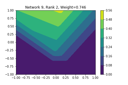
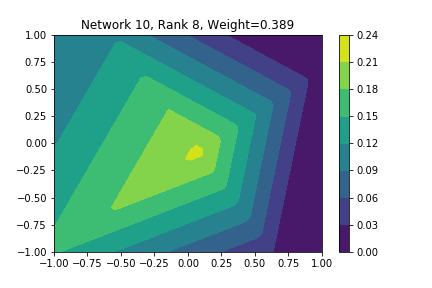
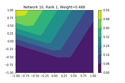
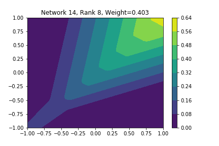
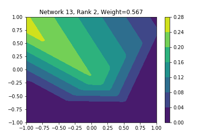
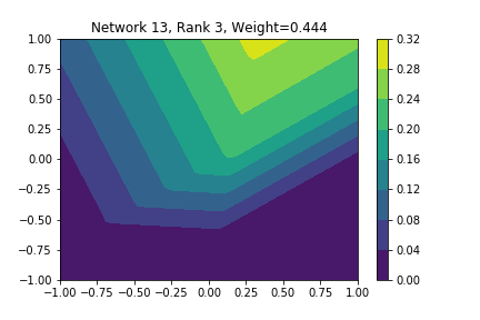
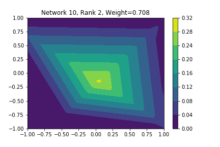
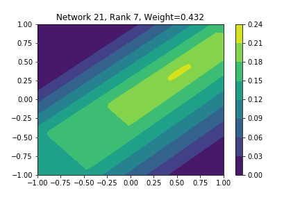
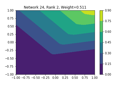
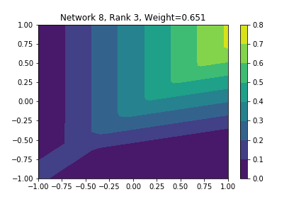
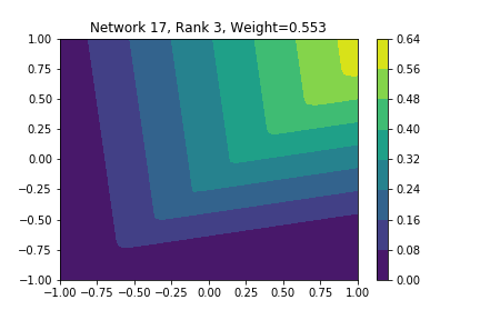
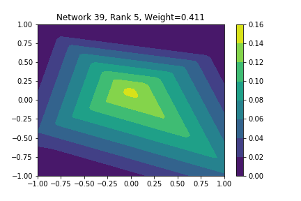
I restricted myself to looking at the quadratic decision boundary since that’s what the manuscript considered. I generated three random integers between 0 and 100 for the seeds of the tensorflow and numpy random number generators. Using all possible combinations of the seeds, I trained networks with 15, 30, and 45 subnetworks on a training set of 2500 samples from a uniform grid on the unit square with a decision boundary given by \( p(x) = x^2 - 0.4 \). I used a batch size of 10 and trained over 10 epochs. After training, the top 10 subnetworks with the largest weights in absolute value in the last layer are graphed in decreasing order. This is the proxy that the manuscript uses to measure the significance of the subnetworks. Here is a table and some figures outlining what I saw.
| NUM_SUBNETS | Numpy Seed | Tensorflow Seed | Notable Shearlet Looking Networks, by Rank |
|---|---|---|---|
| 15 | 47 | 47 | 2, 4, 8, 9, 10 |
| 15 | 47 | 82 | 9, 10 |
| 15 | 47 | 96 | Unremarkable |
| 15 | 82 | 47 | 2, 3, 10 |
| 15 | 82 | 82 | Unremarkable |
| 15 | 82 | 96 | 2, 3, 7, 8 |
| 15 | 96 | 47 | 3, 4, 7 |
| 15 | 96 | 82 | 3, 6 |
| 15 | 96 | 96 | Accuracy < 0.5 |
| 30 | 47 | 47 | 3, 7 |
| 30 | 47 | 82 | 4, 5, 7 |
| 30 | 47 | 96 | 3, 5, 6, 8 |
| 30 | 82 | 47 | 2 |
| 30 | 82 | 82 | 1, 5 (almost) |
| 30 | 82 | 96 | 7 |
| 30 | 96 | 47 | 1, 3, 8 |
| 30 | 96 | 82 | Unremarkable |
| 30 | 96 | 96 | 6 |
| 45 | 47 | 47 | 7 |
| 45 | 47 | 82 | Unremarkable |
| 45 | 47 | 96 | Unremarkable |
| 45 | 82 | 47 | 1, 3, 5, 7 |
| 45 | 82 | 82 | 9, 10 |
| 45 | 82 | 96 | 5 |
| 45 | 96 | 47 | 6, 8 |
| 45 | 96 | 82 | 2, 4 |
| 45 | 96 | 96 | Accuracy < 0.5 |
| 15 Subnetworks | 30 Subnetworks | 45 Subnetworks |
|---|---|---|
 np: 47, TF: 47 np: 47, TF: 47 |
 np: 47, TF: 96 np: 47, TF: 96 |
 np: 82, TF: 47 np: 82, TF: 47 |
 np: 47, TF: 47 np: 47, TF: 47 |
 np: 82, TF: 47 np: 82, TF: 47 |
 np: 82, TF: 47 np: 82, TF: 47 |
 np: 82, TF: 47 np: 82, TF: 47 |
 np: 82, TF: 96 np: 82, TF: 96 |
 np: 82, TF: 82 np: 82, TF: 82 |
 np: 82, TF: 47 np: 82, TF: 47 |
 np: 96, TF: 47 np: 96, TF: 47 |
 np: 82, TF: 96 np: 82, TF: 96 |
I don’t claim that every subnetwork output I marked as being notable is indeed a shearlet. Basically what I was looking for was, as the name suggests, sheared trapezoids. In particular, the manuscript mentions that shearlets “on high scales”, or which are strongly anisotropic, should appear on or near points of singularity; see this and this. By that metric, there were more of these that appeared in the experiments I ran than I expected. To answer the question posed in the title of this blog post, I think that neural networks sometimes learn functions which look like shearlets when you have a quadratic decision boundary. I have some reservations about whether this holds true for general cartoon-like functions. If it were true that learning shearlets for cartoon-like decision boundaries were provably optimal, regardless of network topology, and that cartoon-like functions offer good approximations for natural images, then this greatly undercuts the success of breakthroughs in image classification with deep learning in my opinion.
I think the more interesting point of this manuscript is that neural networks do just as well as representation systems, if not better. The better question to explore is what types of functions are learned by neural networks when they’re trained to approximate a signal class \(\mathcal{C}\). I’m not sure whether we’re equipped mathematically to answer such questions yet. Nevertheless, I think Bölcskei, Grohs, Kutyniok, and Petersen have laid excellent ground work for mathematicians to build off of in answering questions about deep learning.